Dynamic Young‘s Modulus Measurement System (Resonance Method)
Product Overview
The elastic properties of materials under dynamic loading are fundamentally different from those measured under static conditions. Bridges, aircraft wings, and engine components all experience cyclic stresses — making the dynamic measurement of Young’s modulus not just an academic exercise but a practical necessity. The Edusupports Dynamic Young’s Modulus Measurement System (SKU: 0301040041) employs the flexural vibration resonance method to accurately determine Young’s modulus of metallic rods. This approach excites the specimen at its natural frequency and captures the resulting vibration amplitude peak, providing a direct, non‑destructive measurement of material stiffness.
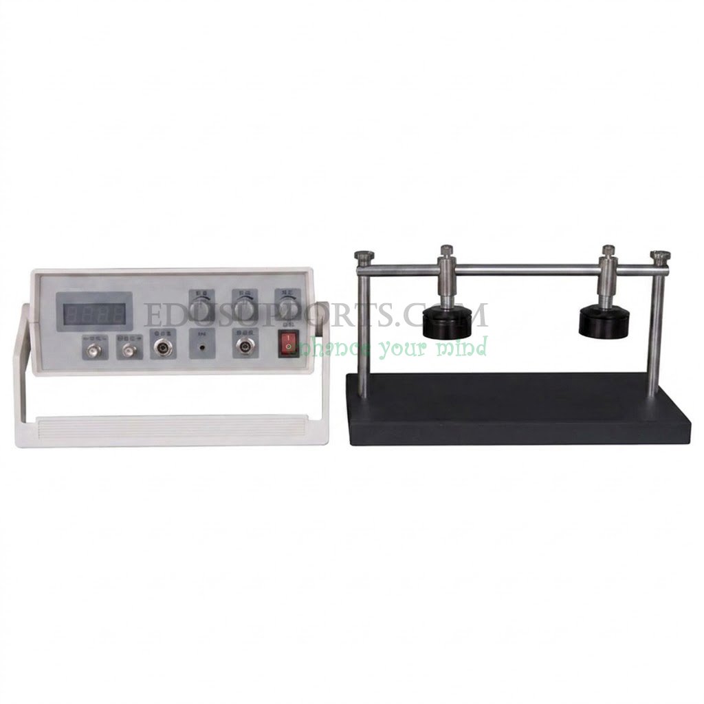
The system is built around three integrated modules:
Precision signal source – Generates a tunable sine wave (200–800 Hz) with 0.1 Hz digital resolution to drive the exciter transducer.
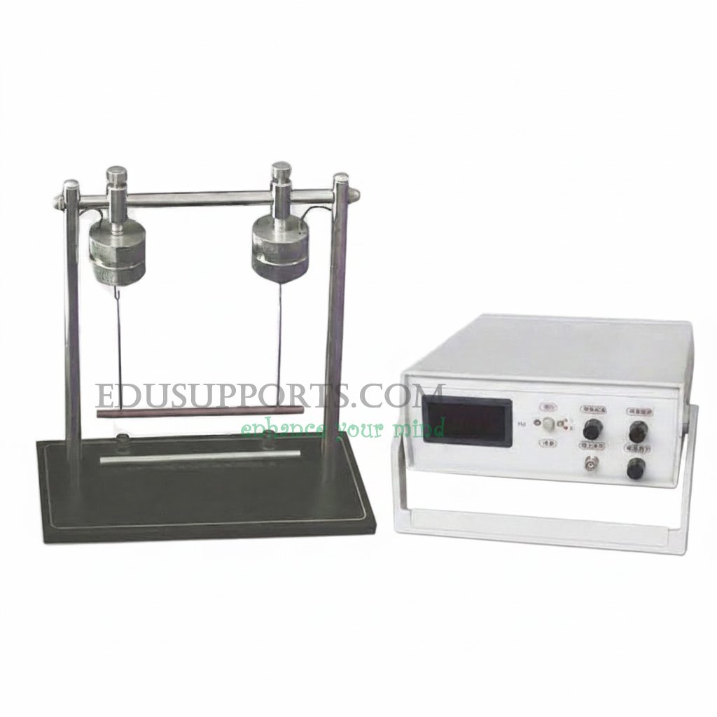
Vibration test platform – Supports both suspending and supporting mounting configurations, with independently adjustable exciter (driver) and pickup (receiver) transducers.
Three calibrated test specimens – Brass (H62), stainless steel, and aluminum rods, each 160 mm long, 6 mm in diameter, and engraved with centimeter markings for accurate positioning.
Using an oscilloscope (user‑supplied), students observe the excitation signal (CH1) and the received resonance signal (CH2). By varying the excitation frequency, they locate the resonant peak, then apply the extrapolation method to eliminate systematic errors caused by placing the exciter and receiver away from the true vibration nodes. The included 50‑page instruction manual provides full theoretical background, step‑by‑step procedures, sample data tables, and error analysis — making this system ideal for undergraduate physics, materials science, and mechanical engineering laboratories.
Key Experiments
| Experiment | Description |
|---|---|
| 1. Fundamental resonance measurement | Mount a brass rod using suspending method; sweep frequency to find resonant peak; calculate Young’s modulus from f_res, mass, length, and diameter. |
| 2. Comparative analysis of three materials | Repeat the procedure for stainless steel and aluminum; compare experimental values with reference data (0.969×10^11, 2.06×10^11, and 0.7×10^11 N/m^2 respectively). |
| 3. Influence of boundary conditions | Perform the same measurement using supporting method (direct contact); discuss how transducer coupling affects resonance frequency and amplitude. |
| 4. Extrapolation method for node correction | For each specimen, measure f_res at seven positions (1,2,3,4,5,6,7 cm from one end); plot frequency vs. position; read the true free‑free resonant frequency at the theoretical node (4.48 cm from each end). |
Core Features
Dual mounting configurations – Suspending method (free‑free beam) and supporting method allow direct comparison of boundary condition effects.
High‑resolution frequency source – 200–800 Hz range, 0.1 Hz digital readout, stable sine wave output.
Sensitive transducers – Exciter (4 ohm, 8 W peak) drives the specimen; pickup (500 ohm) delivers >10 mA signal at resonance without external amplification.
Fully characterised specimens – Brass, steel, aluminium rods with engraved markings at 1,2,3,4,4.48,5,6,7 cm from both ends.
Extrapolation method ready – The engraved marks exactly match the theoretical node position (4.48 cm for a 20 cm rod), enabling accurate node correction.
Oscilloscope compatible – Standard BNC outputs for excitation (CH1) and receiver (CH2) signals; dual‑channel observation of phase and amplitude.
Correction factor table – Provided T1 values for different d/l ratios (0.01–0.10) improve formula accuracy.
Comprehensive manual – Includes Bernoulli‑Euler theory, four resonance identification techniques, sample data for all three materials, and troubleshooting.
Technical Specifications
| Parameter | Value |
|---|---|
| Measurement method | Flexural vibration resonance (dynamic method) |
| Supported configurations | Suspending method / Supporting method |
| Excitation frequency range | 200 Hz – 800 Hz (continuously adjustable) |
| Frequency display | 4‑digit digital panel; resolution 0.1 Hz (100–999.9 Hz) / 1 Hz (1000–9999 Hz) |
| Excitation (drive) voltage | 0 – 10 V adjustable |
| Pickup (receive) output | 0 – 5 V |
| Pickup sensitivity | >10 mA (at 1 V excitation, specimen resonance) |
| Driver impedance | 4 ohm (peak power 8 W, with vibration‑damping soft contact) |
| Receiver impedance | 500 ohm |
| Specimen materials | Brass (H62), Stainless steel, Aluminum |
| Specimen dimensions | Length: 160 mm ±0.5 mm; Diameter: 6 mm ±0.02 mm |
| Specimen markings | Engraved rings at 1,2,3,4,4.48,5,6,7 cm from each end |
| Signal source output power | 600 mW |
| Measurement uncertainty | <3% relative |
| Power supply | AC 220 V, 50 Hz (110 V optional) |
| Test platform dimensions | Approx. 300 x 200 x 150 mm |
| Control unit dimensions | Approx. 200 x 180 x 80 mm |
| Total weight (full set) | ~5 kg |
What’s Included in the Package
| Component | Quantity |
|---|---|
| Vibration test platform (with exciter & pickup transducers, soft‑contact beam holder) | 1 |
| Signal source / electronic control unit (frequency generator, display, gain control) | 1 |
| Brass specimen (H62, 160 mm x 6 mm diameter, graduated) | 1 |
| Stainless steel specimen (160 mm x 6 mm diameter, graduated) | 1 |
| Aluminum specimen (160 mm x 6 mm diameter, graduated) | 1 |
| Connection cables (BNC and multi‑pin) | 4 |
| Support wires and accessories for suspending method | 1 set |
| Full instruction manual (theory, procedures, sample data, correction table) | 1 |
Oscilloscope not included – Any dual‑channel oscilloscope (or a single‑channel with external trigger) can be used; recommended bandwidth ≥20 MHz.
Why Choose This Apparatus?
Lorem ipsum dolor sit amet, consectetur adipiscing elit. Ut elit tellus, luctus nec ullamcorper mattis, pulvinar dapibus leo.
Educational value – Bridges classical beam theory with modern electronic measurement.
Hands‑on learning – Students set up the experiment, adjust frequency, identify resonance, and apply correction factors.
High accuracy – <3% uncertainty when procedures are followed correctly.
Two‑method flexibility – Suspending vs. supporting gives insight into boundary condition effects.
Extrapolation method – Introduces an important experimental technique for eliminating systematic errors.
Cost‑effective – Complete system at an affordable price for teaching laboratories.
Edusupports quality – Robust construction, clear documentation, and responsive technical support.